Tutorials

Running an aquatic ecosystem lake model in R

updated: 06-20-2021

Here’s an updated description of how to run a simple two-layer lake model in R (click this!), which simulates water temperature, dissolved oxygen, phytoplankton, zooplankton and phosphorus dynamics.

Writing a two-layer thermodynamic model in R

updated: 04-16-2020

Introduction

Welcome! In this tutorial, I want to describe and show you how you can write and run a lake model in R. When I began my PhD studies, I had a hard time wrapping my head around all the equations and coding techniques. Therefore, I want to provide a walkthrough here. Please send me an email if you find errors or typos (especially if you find errors!). Hope you enjoy it.

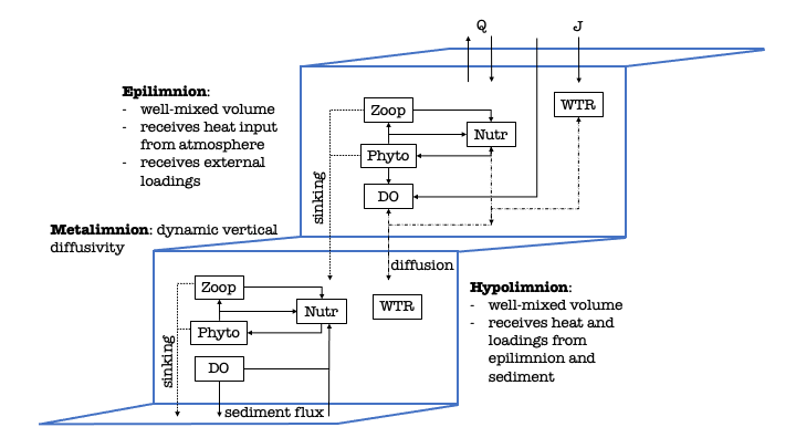
A great type of lake model just assumes that the lake is divided into two volume layers: the epilimnion (surface mixed layer) and the hypolimnion (bottom stagnant layer). Both layers are divided by a metalimnion (layer with a steep density gradient). This model assumption generally holds up for lakes that stratify during the summer. The entrainment over the metalimnion (or thermocline) depends on a vertical diffusion coefficient, which is further simplified as a function of the diffusion at neutral stability to the Richardson number. This last assumption helps the model dynamically change from mixed to stratified conditions.

All equations and derivations are from Steven C. Chapra (2008) ‘Surface Water-Quality Modeling’ Waveland Press, Inc.

Main equations

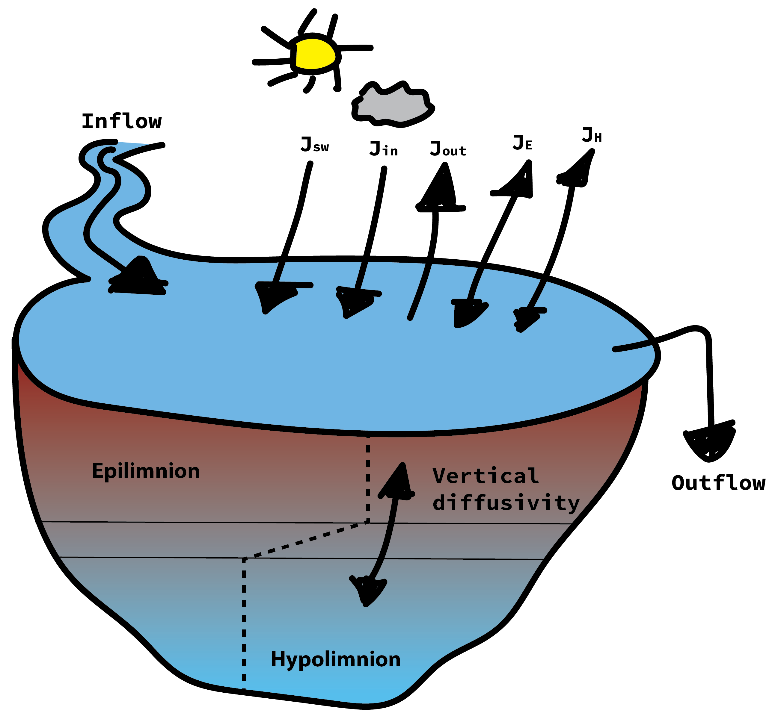
First, we can write the heat balance of the epilimnion as the change of epilimnion water temperature over time in dependence with an inflow source, an outflow sink, turbulent diffusion over the metalimnion between the hypolimnion and epilimnion, as well as heat fluxes from the atmosphere (more to this term later):

In this first ordinary differential equation Q stands for a flow discharge rate, V for different Volumes, for turbulent diffusivity, A for area (index surf for surface area, t for the thermocline area), J for atmospheric heat fluxes, for the density of water, and is the specific heat capacity of water.

Thankfully, the equation for the hypolimnion heat balance is simpler as we are neglecting submerged inflows or sediment heat sources:

How can we get the vertical diffusivity? The goal is to get a dynamic representation of the vertical diffusivity in dependence of the water column stability (in contrast to telling the model to use high or low values on some days). We’ll state the diffusion coefficient as depending on the diffusion at neutral stability to the Richardson number:

We can rewrite the diffusion coefficient at neutral stability to depend on the ratio of wind shear stress to water density:

Here, the wind shear stress depends on the density of the air, a drag coefficient and the measured wind speed:

Next is the Richardson number, which generally describes the work of buoyancy against wind-induced turbulence. If it is below 1/4, the system will experience shear-induced turbulence. It can be estimated by:

where H is the thickness over which the wind can act on the lake (assumed here to be the thermocline depth). Please note that and c are constants.

Boundary and initial conditions

Now we need some boundary conditions to ‘drive’ the model. For this we will use measured daily meteorological data, which will act as heat flux sources from the top (also called Neumann boundary condition type in the literature). We will separate the atmospheric heat fluxes J into (meaning that J is the sum of shortwave radiation, incoming longwave radiation, outgoing longwave radiation, latent heat flux (evaporation), and sensible heat flux (convection and conduction).

We’ll set up each heat flux term now. The easiest one is the solar shortwave radiation, which is ‘just’ the measured shortwave radiation . As the shortwave flux has the unit , we will get a total heat flux (by multiplying with ) of °C/day (this is true for all the other heat fluxes, but I admit that this unit is somehow weird but useful for our simple model). The incoming longwave radiation can be described by (essentially depending on Stefan-Boltzmann constant , air temperature, the air vapor pressure and the reflection). The outgoing longwave radiation from the lake is with being the emissivity of water. The latent heat flux can be calculated with where (function of wind speed) multiplied by the difference between surface water vapor pressure and air vapor pressure. Finally, the sensible heat flux is , here is the Bowen coefficient.

We will assume that the inflow equals the outflow and is constant. Also, the inflow water temperature will be constant. For initial conditions and the sake of simplicity, let’s put the initial water temperature of both layers to 3 °C.

Our model is now looking like this:

How to solve the model

To approximate the solutions of our ordinary differential equations over time, we will use an iterative method called the fourth-order Runge-Kutta method, which has the form: for which we have to solve the coefficients k in dependence of a step-size h>0. Luckily, these numerical methods are included in lots of R packages, for instance deSolve.

Applying the model

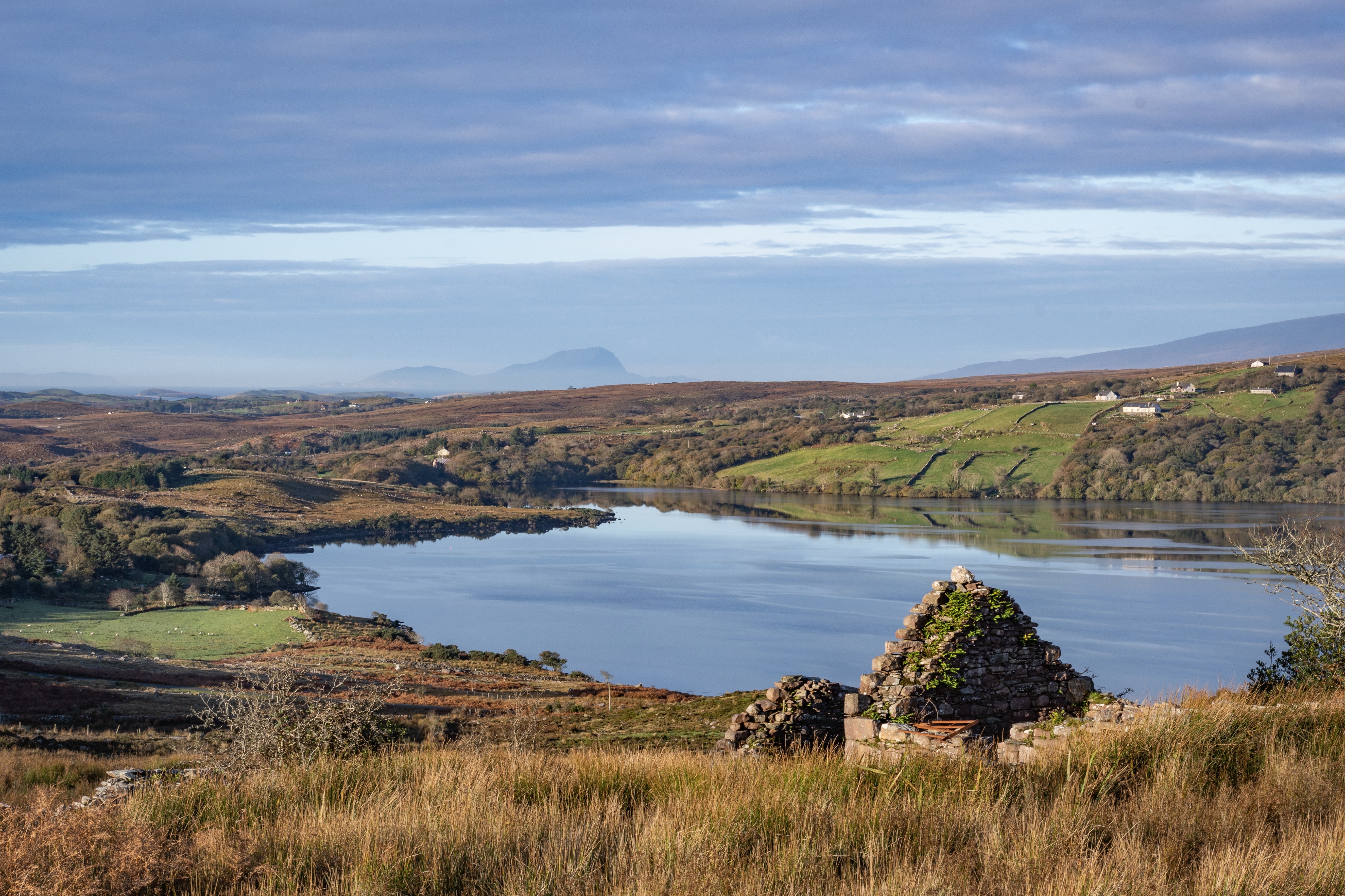
We will try the formulated model on Lough Feeagh in Ireland, which has a maximum depth of 46.8 m. Looks beautiful, right (credits to Mikkel René Andersen):

To run the model, first we need meteorological data, which consists of a time step, the shortwave radiation, the air temperature, the dew point temperature, and the wind speed. You can download the data here.

We also need additional data about the lake which all should be in cm, for instance the volume of the epilimnion (approx. 2.8 10^13 cm3), the volume of the hypolimnion (approx. 3.4 10^13 cm3), the surface area (3.9 10^10 cm2), the thermocline area (2.6 10^10 cm2), and the thickness of the metalimnion (let us assume it to be about 300 cm). We will neglect any inflows and outflows for this example (this simplifies our model even more, awesome!). Next we have to estimate the depth of the thermocline. For this we will use a regression from Hanna M. (1990): Evaluation of Models predicting Mixing Depth. Can. J. Fish. Aquat. Sci. 47: 940-947:

This means that the thermocline depth depends on the maximum distance over our lake (either length or width). We need this depth to estimate our volumes (epilimnion and hypolimnion) and the respective areas (thermocline area) from bathymetry data if we don’t know it a priori.

Now it’s the perfect time to load our libraries:

library(gridExtra)
library(ggplot2)
library(pracma)
library(tidyverse)
library(RColorBrewer)
library(zoo)
library(deSolve)

Let us first state the important parameters, load the data and give the model some initial conditions:

# load in the boundary data
urlfile = "https://raw.githubusercontent.com/robertladwig/robertladwig.github.io/master/files/meteo.txt"
bound <- read_tsv(url(urlfile))

# approximate the thermocline depth
therm_depth <- 10 ^ (0.336 * log10(3678) - 0.245) 
simple_therm_depth <- round(therm_depth)

Ve <- 2.886548e+13 # epilimnion volume (cm3)
Vh <- 3.421416e+13 # hypolimnion volume (cm3)
Ht <- 3 * 100 # thermocline thickness (cm)
At <- 26850835487 # thermocline area (cm2)
As <- 3.931e+10 # surface area (cm2)
Tin <- 0 # inflow water temperature
Q <- 0 # inflow discharge 
Rl <- 0.03 # reflection coefficient (generally small, 0.03)
Acoeff <- 0.6 # coefficient between 0.5 - 0.7
sigma <- 11.7 * 10^(-8) # cal / (cm2 d K4) or: 4.9 * 10^(-3) # Stefan-Boltzmann constant in (J (m2 d K4)-1)
eps <- 0.97 # emissivity of water
rho <- 0.9982 # density (g per cm3)
cp <- 0.99 # specific heat (cal per gram per deg C)
c1 <- 0.47 # Bowen's coefficient
a <- 7 # constant
c <- 9e4 # empirical constant
g <- 9.81  # gravity (m/s2)
thermDep <- simple_therm_depth

parameters <- c(Ve, Vh, At, Ht, As, Tin, Q, Rl, Acoeff, sigma, eps, rho, cp, c1, a, c, g, thermDep)

colnames(bound) <- c('Day','Jsw','Tair','Dew','vW')

# function to calculate wind shear stress (and transforming wind speed from km/h to m/s)
bound$Uw <- 19.0 + 0.95 * (bound$vW * 1000/3600)^2 
bound$vW <- bound$vW * 1000/3600

boundary <- bound

# simulation maximum length
times <- seq(from = 1, to = max(boundary$Day), by = 1)
# initial water temperatures
yini <- c(3,3) 

Great, now we write down the model itself as a function (which you can also find here):

run_model <- function(bc, params, ini, times){
  
  Ve <- params[1]
  Vh <- params[2]
  At <- params[3]
  Ht <- params[4]
  As <- params[5]
  Tin <- params[6]
  Q <- params[7]
  Rl <- params[8]
  Acoeff <- params[9]
  sigma <- params[10]
  eps <- params[11]
  rho <- params[12]
  cp <- params[13]
  c1 <- params[14]
  a <- params[15]
  c <- params[16]
  g <- params[17]
  thermDep <- params[18]
  
  TwoLayer <- function(t, y, parms){
    eair <- (4.596 * exp((17.27 * Dew(t)) / (237.3 + Dew(t)))) # air vapor pressure
    esat <- 4.596 * exp((17.27 * Tair(t)) / (237.3 + Tair(t))) # saturation vapor pressure
    RH <- eair/esat *100 # relative humidity
    es <- 4.596 * exp((17.27 * y[1])/ (273.3+y[1]))
    # diffusion coefficient
    Cd <- 0.00052 * (vW(t))^(0.44)
    shear <- 1.164/1000 * Cd * (vW(t))^2
    rho_e <- calc_dens(y[1])/1000
    rho_h <- calc_dens(y[2])/1000
    w0 <- sqrt(shear/rho_e) 
    E0  <- c * w0
    Ri <- ((g/rho)*(abs(rho_e-rho_h)/10))/(w0/(thermDep)^2)
    if (rho_e > rho_h){
      dV = 100
    } else {
      dV <- (E0 / (1 + a * Ri)^(3/2))/(Ht/100) * (86400/10000)
    }
    
    # epilimnion water temperature change per time unit
    dTe <-  Q / Ve * Tin -              # inflow heat
      Q / Ve * y[1] +                   # outflow heat
      ((dV * At) / Ve) * (y[2] - y[1]) + # mixing between epilimnion and hypolimnion
      + As/(Ve * rho * cp) * (
        Jsw(t)  + # shortwave radiation
          (sigma * (Tair(t) + 273)^4 * (Acoeff + 0.031 * sqrt(eair)) * (1 - Rl)) - # longwave radiation into the lake
          (eps * sigma * (y[1] + 273)^4)  - # backscattering longwave radiation from the lake
          (c1 * Uw(t) * (y[1] - Tair(t))) - # convection
          (Uw(t) * ((es) - (eair))) )# evaporation
    
    # hypolimnion water temperature change per time unit
    dTh <-  ((dV * At) / Vh) * (y[1] - y[2]) 

    # diagnostic variables for plotting
    mix_e <- ((dV * At) / Ve) * (y[2] - y[1])
    mix_h <-  ((dV * At) / Vh) * (y[1] - y[2]) 
    qin <- Q / Ve * Tin 
    qout <- - Q / Ve * y[1] 
    sw <- Jsw(t) 
    lw <- (sigma * (Tair(t) + 273)^4 * (Acoeff + 0.031 * sqrt(eair)) * (1 - Rl))
    water_lw <- - (eps * sigma * (y[1]+ 273)^4)
    conv <- - (c1 * Uw(t) * (y[1] - Tair(t))) 
    evap <- - (Uw(t) * ((esat) - (eair)))
    Rh <- RH
    E <- (E0 / (1 + a * Ri)^(3/2))
    
    write.table(matrix(c(qin, qout, mix_e, mix_h, sw, lw, water_lw, conv, evap, Rh,E, Ri, t), nrow=1), 'output.txt', append = TRUE,
                quote = FALSE, row.names = FALSE, col.names = FALSE)

    return(list(c(dTe, dTh)))
  }
  
  # approximating all boundary conditions  (linear interpolation)
  Jsw <- approxfun(x = bc$Day, y = bc$Jsw, method = "linear", rule = 2)
  Tair <- approxfun(x = bc$Day, y = bc$Tair, method = "linear", rule = 2)
  Dew <- approxfun(x = bc$Day, y = bc$Dew, method = "linear", rule = 2)
  Uw <- approxfun(x = bc$Day, y = bc$Uw, method = "linear", rule = 2)
  vW <- approxfun(x = bc$Day, y = bc$vW, method = "linear", rule = 2)
  
  # runge-kutta 4th order
  out <- ode(times = times, y = ini, func = TwoLayer, parms = params, method = 'rk4')
  
  return(out)
}

As you can see in the code, the function reads in your boundary conditions, the parameters, the initial conditions and the run time. Then for simplicity it assigns these values to variables. The model itself is written as a separate function INSIDE the function which takes the run time, the initial values and the parameters as input. This sub-function then calculates important variables for every time step, e.g. air vapor pressure, air saturation, the diffusion coefficient, shear stress, water densities and the vertical diffusivity (we assume the lake is completely mixed during fall to spring, therefore the value becomes 100). Then you can see the two differential equations. At the end I added some lines to write the fluxes and variables into a separate text file, which we can use to investigate the model performance. Before the model is run (using Runge-Kutta), we need to interpolate the meteorological data (because the time steps can be below a day).

And another small function to calculate water density from temperature:

calc_dens <- function(wtemp){
  dens = 999.842594 + (6.793952 * 10^-2 * wtemp) - (9.095290 * 10^-3 *wtemp^2) + (1.001685 * 10^-4 * wtemp^3) - (1.120083 * 10^-6* wtemp^4) + (6.536336 * 10^-9 * wtemp^5)
  return(dens)
}

Now it’s time … exciting, right?

out <- run_model(bc = boundary, params = parameters, ini = yini, times = times)

If you don’t get any warning, that’s good! Now we can look at the model output which is stored in the variable “out”:

result <- data.frame('Time' = out[,1],
                     'WT_epi' = out[,2], 'WT_hyp' = out[,3])
g1 <- ggplot(result) +
  geom_line(aes(x=Time, y=WT_epi, col='Surface Mixed Layer')) +
  geom_line(aes(x=(Time), y=WT_hyp, col='Bottom Layer')) +
  labs(x = 'Simulated Time', y = 'WT in deg C')  +
  theme_bw()+
  guides(col=guide_legend(title="Layer")) +
  theme(legend.position="bottom")

output <- read.table('output.txt')

output <- data.frame('qin'=output[,1],'qout'=output[,2],'mix_e'=output[,3],'mix_h'=output[,4],
                     'sw'=output[,5],'lw'=output[,6],'water_lw'=output[,7],'conv'=output[,8],
                     'evap'=output[,9], 'Rh' = output[,10],
                     'entrain' = output[,11], 'Ri' = output[,12],'time' = output[,13])

output$balance <- apply(output[,c(1:9)],1, sum)

g2 <- ggplot(output) +
  geom_line(aes(x = time,y = qin, col = 'Inflow')) +
  geom_line(aes(x = time,y = qout, col = 'Outflow')) +
  geom_line(aes(x = time,y = mix_e, col = 'Mixing into Epilimnion')) +
  geom_line(aes(x = time,y = mix_h, col = 'Mixing into Hypolimnion')) +
  geom_line(aes(x = time,y = sw, col = 'Shortwave')) +
  geom_line(aes(x = time,y = lw, col = 'Longwave')) +
  geom_line(aes(x = time,y = water_lw, col = 'Reflection')) +
  geom_line(aes(x = time,y = conv, col = 'Conduction')) +
  geom_line(aes(x = time,y = evap, col = 'Evaporation')) +
  geom_line(aes(x = time,y = balance, col = 'Sum'), linetype = "dashed") +
  scale_colour_brewer("Energy terms", palette="Set3") +
  labs(x = 'Simulated Time', y = 'Fluxes in cal/(cm2 d)')  +
  theme_bw()+
  theme(legend.position="bottom")

g3 <- ggplot(output) +
  geom_line(aes(x = time,y = Ri, col = 'Richardson')) +
  geom_line(aes(x = time,y = entrain, col = 'Entrainment')) +
  scale_colour_brewer("Stability terms", palette="Set1") +
  labs(x = 'Simulated Time', y = 'Entrainment in cm2/s and Ri in [-]')  +
  theme_bw()+
  theme(legend.position="bottom")

g4 <- ggplot(boundary) +
  geom_line(aes(x = Day,y = scale(Jsw), col = 'Shortwave')) +
  geom_line(aes(x = Day,y = scale(Tair), col = 'Airtemp')) +
  geom_line(aes(x = Day,y = scale(Dew), col = 'Dew temperature')) +
  geom_line(aes(x = Day,y = scale(vW), col = 'Wind velocity')) +
  geom_line(aes(x = Day,y = scale(Uw), col = 'Wind shear stress')) +
  scale_colour_brewer("Boundary Conditions", palette="Set3") +
  labs(x = 'Simulated Time', y = 'Scaled meteo. boundaries')  +
  theme_bw()+
  theme(legend.position="bottom")

g5 <- grid.arrange(g1, g2, g3, g4, ncol =1);g5

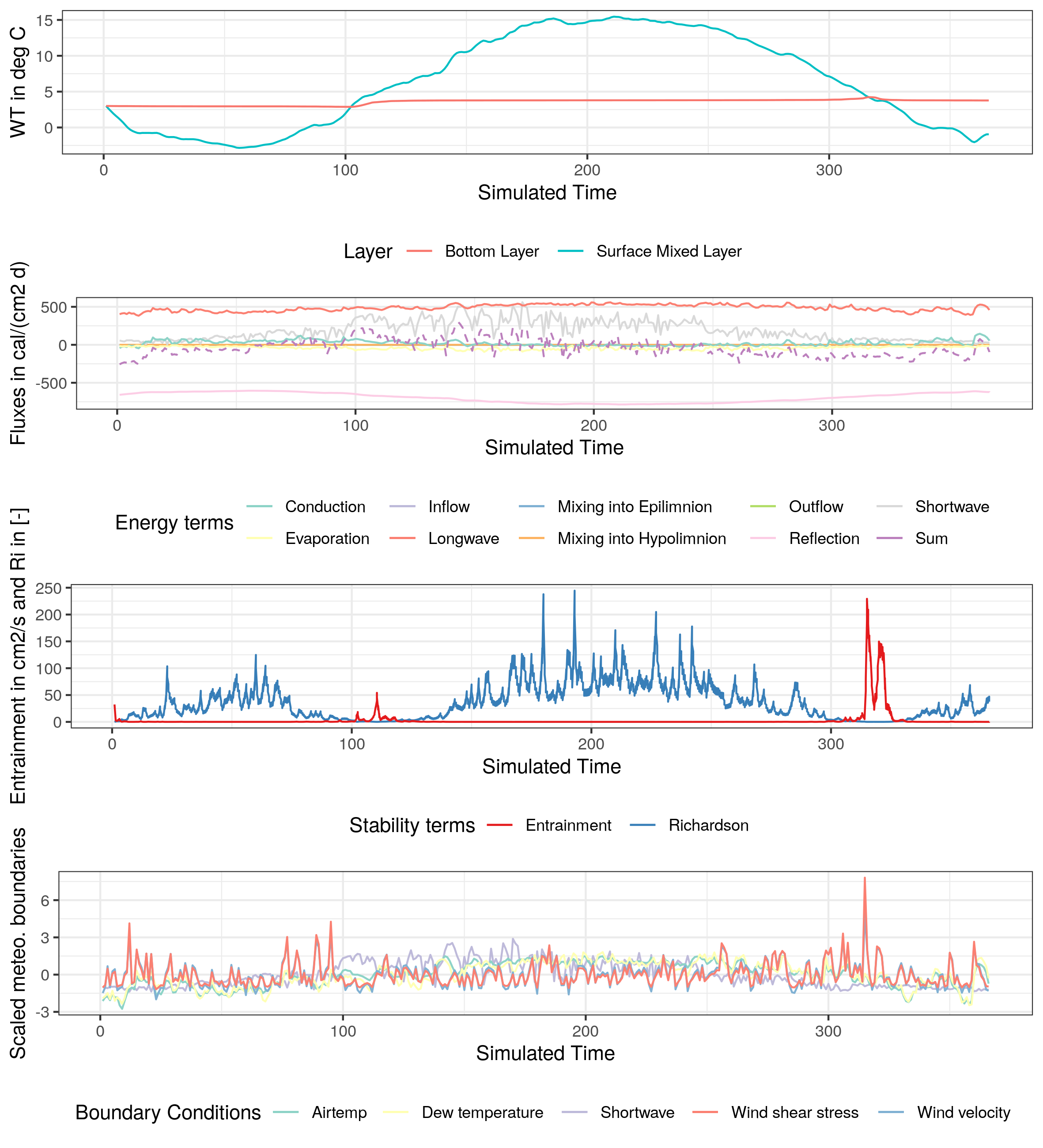
And the results look surprisingly reasonable. The lake warms up during summer, cools down in winter, has high Richardson numbers during summer, and the heat fluxes have nice seasonal dynamics. Not too bad.

Let’s compare how well our model compares to reality. In the next plot red symbolizes the surface layer and blue the bottom layer. Also, solid lines are model results and dashed lines are observed data (measured at 0.9 and 42 m, respectively).

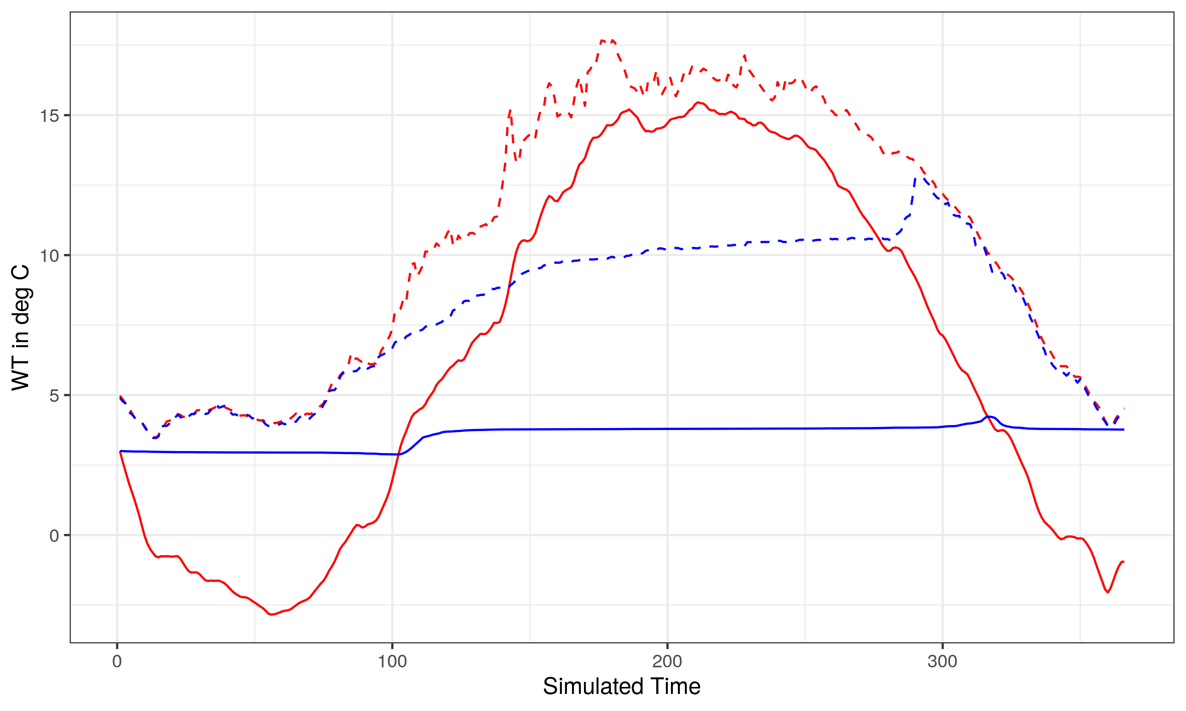
Okaaay, it’s doing some parts well, some parts bad. But keep in mind that the model is not calibrated yet (we assumed several parameters), doesn’t include any inflow dynamics, vertical mixing is vastly simplified, and the observed data wasn’t vertically averaged.

Final thoughts

I hope this tutorial was helpful in explaining how a two-layer lake model can be coded in R. Of course, the code could be more efficient, faster and better looking, but I wanted to give you a short walkthrough on how to do it once you have all the important equations. Mathematical modeling can sound scary at the beginning, but once your code is working all pain will be forgotten.